Cobordic Quantum Computing: Defining Logical Computation through Manifold Geometry
Beyond NISQ
“Today the physicist sacrifices structural stability for computability. I hope that he will not have cause to regret this choice."
— René Thom (The Founder of Cobordism)
"We can view any cobordism M between S0 and S1 as inducing a linear transformation between their respective Hilbert spaces."
- Michael Atiyah (Cobordism in Quantum Field Theory)
“It is very possible that a proper understanding of string theory will make the space-time continuum melt away.”
— Edward Witten (Cobordism and the Nature of Reality)
“It is most natural to suppose that the entropy of a black hole is proportional to the area of its horizon.”
“The entropy of a black hole measures the amount of information about the physical state of matter which is hidden from an outside observer.”
— Jacob Bekenstein
The Quantum
Computing (QC) has been a
topic of interest for quite
a while now. However
while the working prototypes
exist, the general-purpose
machines are decades away,
even in the most optimistic
scenario. In essence,
QC is in the same state as
the digital computing was
back in 1950s.
At present, QC is in what is
known as Noisy
Intermediate-Scale Quantum
(NISQ) era. The
scaling in NISQ is limited
to 1000 quantum gates,
exceeding which the noise
inherent in quantum
circuits, accumulates to
overwhelm the original
signal rendering computation
meaningless.
Our objective in
forthcoming blogs, is to
discuss the limitations in
existing QC landscape, which
must be overcome to take QC
to the next level. The
areas we will be interested
in are:
1. Qubit
architecture/Hardware:
Moving beyond fragile
qubits.
2. Algorithms:
Designing for topological
stability.
3. Software: Compiling
for geometric structures.
4. Applications:
Identifying where
"shape-based" logic
outperforms linear algebra.
We have already discussed QC
at a very elementary level earlier.
Almost a decade down the
line, now our main
focus however, is on what we
think a logical computing
really means in terms of
manifolds. And to be
very frank, we do not
know what our findings will
be in either of four
categories mentioned above.
There are
examples of highly
sophisticated Topological
Quantum Computers,
which are the physical
hardware built from
topological phases. In this
case the manifolds are
braided together to complete
a surface.
Cobordism
allows us to mathematically
approach this problem in a
quite different
manner. We want to
understand how Cobordism
relates two different
boundary states and how it
acts as the engine behind a
logical computation.
In a sense, we are more
interested in the actual
geometry behind manifolds
and how it relates to the
logical computation.
The fundamental equation behind Cobordic Quantum Computing (CQC) can be stated a follows:
Boundary Hilbert Spaces are the vector spaces of quantum states that live on the edge (boundary) of a physical region. For example, gravity in a volume (the bulk) is mathematical dual to a quantum field theory living on its boundary.
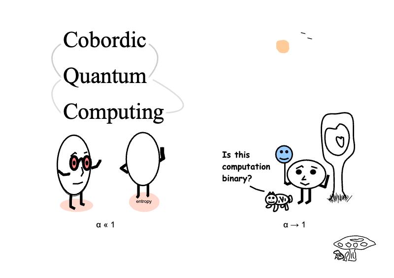
However, the important point to note is that the boundary itself is not a conventional 1-dimensional boundary. The boundary can be either 3D or n-dimensional whereas the bulk is then 4D or n+1-dimensional respectively. In j-space, the "bulk" is the logic while the "boundary" is the data or observable(s), as measured by a finite capability observer ( < 1).1
The simplest example to visualize CQC mechanism, is the event-horizon of a black-hole. In Beckenstein-Hawkings view, all the information contained within a black-hole (3D bulk) is encoded on its 2D surface i.e. event-horizon. The event-horizon is the null surface defined by the light-like (null) geodesics.
As another example, we can think of a soap bubble, where the surface is the thin-film and bulk is represented by volume of the air trapped inside. In conventional QC, the thin film is manipulated bit-by-bit using time-evolution. However in CQC, the bulk is mathematically constrained to change, based on the information placed on the surface.
Replace this picture of bulk with space-time. When the information on the surface is changed, the space-time is mathematically constrained (cobordism) to move to next state as the information on the surface and the bulk must be aligned to satisfy General Relativity.2 And this is the mechanism behind the logical computation in CQC.
We note that in essence we are constraining the manifold to permissible solutions in space-time. A summary of the comparison between standard Quantum Computing and CQC is provided below:

The fundamental idea behind the algebraic geometry is that, "All the geometric information of a space can be encoded in the algebraic structures." The simplest example is that a circle (geometry) can be written as (algebra).
In topology, we enhance this idea to include the "connectivity" of the "spaces". Before we write algebra, we must decide if the shapes are topologically equivalent. Often quoted example, is that a doughnut and a coffee mug are topologically equivalent to each other as their Euler characteristics are the same. This enhancement is extremely important as we study the underlying structure (bulk) before we launch into writing complicated equations (boundaries). (Arguably, the algebraic equation of a torus is much simpler than that for a coffee mug.)
We can think of CQC as the following categories:
1. Physical hardware built from topological phases
2. Logical computation defined as cobordism between boundary states
The category-1 refers to, refers to quantum computing platforms where information is stored and manipulated using the global topological properties of a material, rather than fragile local states like individual electron spin or photon polarization.
In certain exotic materials—such as topological superconductors or fractional quantum Hall systems—quasiparticles called anyons can appear. When these anyons are moved (or braided) around each other, the system’s quantum state changes in a way that depends only on the topological pattern of the braid, not on the exact path taken or small environmental disturbances. Because topology is insensitive to small errors, this approach naturally protects quantum information from noise and decoherence.
In practice, the “hardware” consists of engineered materials and nanostructures where these topological excitation can be created, moved, and measured, turning braiding patterns into quantum logic operations. This idea underlies topological quantum computing, pursued experimentally in systems like fractional quantum Hall devices, Majorana zero modes in superconducting nanowires, and other strongly correlated quantum materials.
However, our focus is on CQC category-2. The logical computation defined as cobordism between boundary states, is a viewpoint where a computation is not described as a sequence of time-ordered gates acting on qubits, but as a single geometric object connecting an initial state and a final state.
In topology, a cobordism is a higher-dimensional space whose boundary consists of two lower-dimensional shapes. Translating this idea to computation, the input state and output state are treated as boundaries, and the entire computation is the bulk structure that connects them. The logical transformation is therefore determined by the global properties of this connecting space rather than by step-by-step operations. A simple example is a cylinder whose two ends are connected through a higher dimensional bulk.

Different possible “fillings” or geometries between the same boundaries can contribute phases or transformations, much like path integrals in quantum physics. This perspective shifts the focus from local gate operations to global topology, allowing computation to be understood as a relationship between boundary states mediated by an allowed geometric bridge.
We will be discussing next, some basic concepts related to the Cobordic Quantum Computing in the discrete measurement space or j-space. It will be followed by Michael Atiyah axioms for a Topological Quantum Field Theory (TQFT), which formalize how cobordisms act as “processes” connecting spaces. The key idea is that "a TQFT assigns algebraic objects to spaces and linear maps to cobordisms and therefore geometry algebra."
2. The geometric quantities on the LHS of Einstein's equations (the Einstein tensor ) are effectively encodings of the information density stored in the Boundary Hilbert Space ().

An Ecosystem of δ-Potentials - III
An Ecosystem of δ-Potentials - II
An Ecosystem of δ-Potentials - I
Nutshell-2019
Stitching Measurement Space - III
Stitching Measurement Space - II
Stitching Measurement Space - I
Mass Length & Topology
A Timeless Constant
Space Time and Entropy
Nutshell-2018
Curve of Least Disorder
Möbius & Lorentz Transformation - II
Möbius & Lorentz Transformation - I
Knots, DNA & Enzymes
Quantum Comp - III
Nutshell-2017
Quantum Comp - II
Quantum Comp - I
Insincere Symmetry - II
Insincere Symmetry - I
Existence in 3-D
Infinite Source
Nutshell-2016
Quanta-II
Quanta-I
EPR Paradox-II
EPR Paradox-I
De Broglie Equation
Duality in j-space
A Paradox
The Observers
Nutshell-2015
Chiral Symmetry
Sigma-z and I
Spin Matrices
Rationale behind Irrational Numbers
The Ubiquitous z-Axis

Attribution — You must give appropriate credit, provide a link to the license, and indicate if changes were made. You may do so in any reasonable manner, but not in any way that suggests the licensor endorses you or your use. No additional restrictions — You may not apply legal terms or technological measures that legally restrict others from doing anything the license permits. This is a human-readable summary of (and not a substitute for) the license.
