ijspace: Surface of least energy

    We have described earlier the constraint of existence in 3-D in the macroscopic observer's, Obs_M , measurement frame, i.e. coordinate time frame. There we had mentioned how the stability of the structures was dependent upon the formation of the least energy surfaces. The energy plays an important role in our everyday life. However in essence, the conventional energy is equivalent to the disordered information ¹. Thus the formation of least energy surfaces, is equivalent to the formation of the surfaces with an objective to minimize the disorder.

The formation of the least-energy or least-disorder surface, is important as it provides us with the knowledge of the geometric structure of the infinitesimal volume element dV_j of the measurement metric. The fundamental geodesic of measurement used by the electron-photon interaction or Obs_c, will lie on dV_j. The surface dV_j could be spherical, ellipsoidal, or any other shape. The surfaces formed are likely to be in Planck's dimensions. We will be discussing the criterion to form these surfaces in one dimension. The argument, can be generalized to any multi-dimensional manifold.

The energy corresponding to a curve passing through two neighbouring points with the arc length ds, is given as:

E = ∫ κ² ds,

where κ is the curvature of the arc, and it is related to the radius of the arc ρ as, κ = 1/ρ. Therefore for a pure point, the curvature is infinite and the radius is zero. Similarly for a precise straight line the curvature is zero, and hence the radius is infinite.

The simplest case to consider, is when a curve is completed using a single arc. The curve of least-energy, is a circle and the corresponding least-energy surface is the surface of a sphere. In ideal discrete measurement space, no two measurements are alike. Consequently each ds, is of different curvature and different radii. If we plot a curve using same origin as reference, we run into a rather serious problem, as shown below:

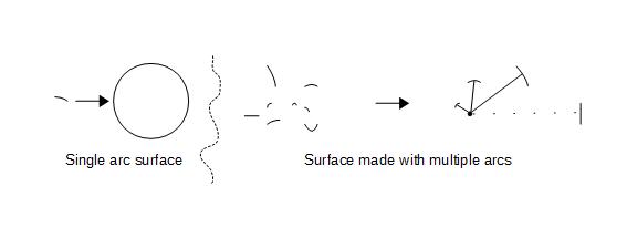
The curve on left, is formed using a single arc. In this case when arcs are connected with respect to the same origin, a smooth curve i.e. a circle is formed, which is the curve of least-energy or the curve of least-disorder in this case. A real life example, is the surface formed by a soap bubble. However the situation in Planck's domain, is likely to be a little bit more complicated. As shown on the right in the picture above, if we try to connect arcs of varying curvatures using the same origin, a "smooth" curve can not be formed. An approach to solve this problem, is as following:

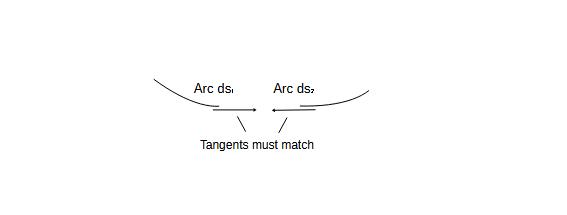
We connect two arcs ds₁ and ds₂, whose tangents at the end points are infinitesimally close to each other in their values. Now we can proceed to complete the curve, by connecting another arc-ds₃ to the arc-ds₂ in similar fashion, and so on. Thus we can form a path by joining a large number of curves, based on the criterion of connecting closest matching tangents. Now we have a range of familiar geometric figures as possible solutions, to the problem of forming the curve of least-disorder. They are shown below:

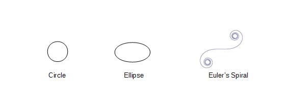
These shapes appear in various phenomena in nature, however which one of them corresponds to the curve of least-disorder when the number of arcs approaches infinity, is not very obvious. To determine the nature of the infinitesimal volume dV_j, we have to find the geometric shape as the number of arcs approach ∞_j. The energy stored in a semicircle of unit radius, number of arcs = 1, can easily shown to be π/2. As the number of arcs is increased, the amount of energy stored in the curve can be shown to be decreasing. These values are shown below²:

Geometry	No. of Arcs	Total Energy
Circle	1	1
Ellipse	2	.9342
	3	0.927478
	4	0.9219604
	5	0.9192345
	6	0.9176931
	-	-
	-	-
	-	-
	64	0.913953
Euler's Spiral	-	0.9178877
Limiting Value	∞	0.9138931623

As it can be seen neither of the known curves i.e. Circle, Ellipse, and Euler's Spiral, correspond to the curve of least-energy. Furthermore as the number of arcs is increased towards infinity, the energy contained within the curve keeps decreasing until it hits the limit of approximately 91.39% of the energy, π/2, stored in a semicircle. These values are calculated using the multi-arc approximation. Analytically, the n -> ∞j situation is represented by Cesaro form, using Whewell equation which correlates the arc length to the tangential angle. The arc-length and the corresponding energy, using Gamma function are given as:

In discrete measurement space, the appearance of the Gamma function is always a good sign, because of the presence of the term e^-q (eqn. iv). This also means that Beta function can not be far behind. Let us consider the coordinate differential ds², defined in General Theory of Relativity as:

ds² = g_μν x^μ x^ν,

where the value of ds² depends upon the metric tensor g_μν. The curve of least-disorder, provides a method to estimate ds itself. Since ds is equivalently the curve of least energy, it will be an invariant. The requirements for the invariance of ds, are much more strict than those for ds².

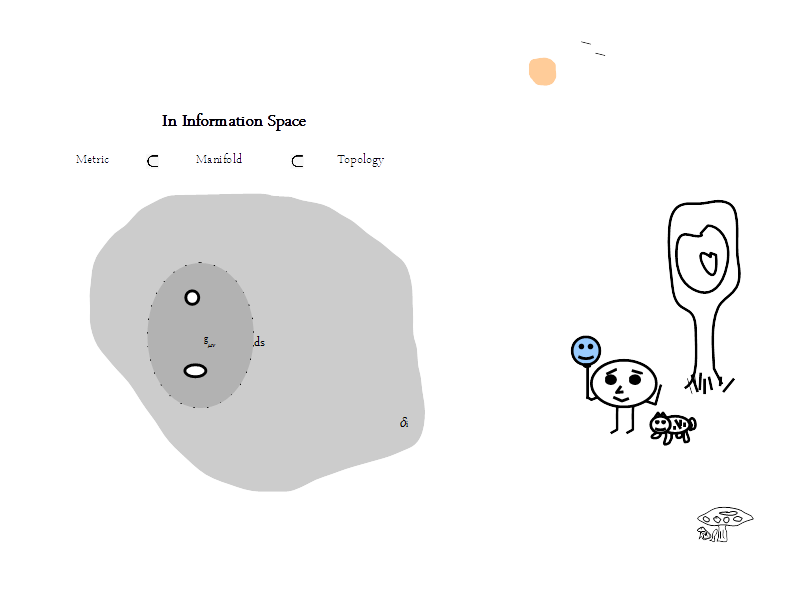
We note that in j-space we are measuring the information space itself, with no assumption made about the nature of the information, such as known physical objects or any other known phenomenon. We are discussing here, the formation of a manifold from which the metric in observer's measurement space is derived. The relationship between the topology, the manifold, and the metric is shown here:

LES 5

The topological space in this case is defined by δ_i. The curve of least-energy represents the manifold corresponding to the measurements made by an observer of maximum efficiency Obs_c (v/c ~ 1). The metrics in various observers' measurement systems, are given by respective g_μν's and g_mn's. We should also mention that the problem of the curve of least-energy or least-disorder, is equivalent to the problem of the resource optimization in j-space, which we have discussed earlier.

The curve of least-disorder provides a solution for the problem of the origin in the discrete measurement space or j-space, in a most satisfactory manner. The origin is defined in the manifold using a least-disorder curve and then coordinate systems are developed in various metric spaces, based on this definition of origin. In other words, the measurements in the j-space, can be performed based on the value of ds, which is finite with the least-disorder criterion, and in essence defines the value of 0_j for various measurement metrics.

The curve of least-disorder ds, is independent of the coordinate frames which require complicated metric tensors to determine the coordinate differential ds². More importantly, ds brings us closer to the underlying topological space, which governs the formation of the structures at cosmic as well as Planck scales.