Higglety
pigglety
Robert A. Millikan
Scrutinized oil drops
And so measured e;
Studied phenomena
Photoelectrical,
Won the Nobel Prize and
Said ‘Look at ME!"
-
Professor A. P. French.
"A proton
once said, "I'll fulfill
My long-term belief in free will.
Though theorists (may) say
That I ought to decay
I'm damned if I think that I will."
- Proton Decay by David Halliday.
The first law
of Newton I sing
My voice has a relevant ring:
"An object left free
Of hassles will be
Engrossed in just doing its thing."
- Doin' its Own Thing by Edward H.
Green.
Miss
Farad was pretty and sensual
And
charged to a reckless potential;
But a
rascal named Ohm
Conducted
her home -
Her
decline was, alas, exponential.
- Condensed Story of Ms Farad
by A. P.
French.
On a merry-go-round in the night,
Coriolis was shaken with fright.
Despite how he walked,
'Twas like he was stalked,
By some fiend always pushing him right.
- May the Force Be With You
by David Morin, Eric Zaslow, E'beth Haley, John Golden, and Nathan Salwen.
***
We discussed in the previous blog that:
- We need resources even for a zero-entropy measurement.
- Simplest method "COUNTING".
- We build a picture by completing various circuits in j-space, add them up, and then fill in details based on the a priori knowledge, where a priori knowledge ≡ initial state <t = 0j>.
- Measurements require the presence of a field.
- In j-space for each point in space-time field, a system must have both tangential and normal components.
- To above we further add that, the Theory of Special Relativity and Anharmonic Coordinates play an important role in j-space.
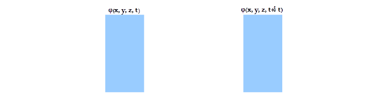
Let us first describe physical picture behind the measurements as they are made in conventional (t, x, y, z) metric, used by Aku. Consider the following description of field φ at a point (x, y, z) at time instants t and t+δt.
We note that when we make the statement that a field exists in the measurement space, we acknowledge the existence of the tangential component of the system. The normal component or the structure part of the system is assumed to exist, but it is not the part of the field description. This is an important point to understand. The system in essence, is an infinite source which is being measured. When the normal component (i.e. memory of the initial state <t = 0j>) is assumed to exist, it is scalar in nature, whereas the field itself is a vector field described by the tangential component.
The picture is similar to the quaternion structure, but with an important difference. We note that the information content within the tangential field or a vector field, is much smaller than that of the normal component of the system or a scalar field. We can visualize this description in the form of a Hydrogen atom, where an electron is in the orbit of a proton. We can easily set up any tangential field based on electrons alone.
While describing this electric or electromagnetic field, the description of proton is not necessary. Yet when we describe the whole system, protons are also included and consequently energy-scales shift by many orders of magnitude. The discussion in this blog, refers to fields due to tangential components only. The memory of the initial state <t = 0j> will be accounted for later, when we bring in anharmonic coordinates in the description of j-space.
When we say that a field is established, in essence we are making following statements, which are true for every time instant in Aku's frame of reference:
- The origin 0j is established in the measurement space based on VT-symmetry, by Obsc.
- The curve of least disorder, can be measured, i.e. all the arcs forming the the curve of least disorder can be precisely measured by Obsc. (Aku is represented by ObsM.)
- Lorentz Transformation is obeyed by all measurements made by Aku. The locality condition hold.
- The structures measured by Aku are conformal and Möbius transformations apply between the structures. We should note that conformity allows for an unique unit normal vector for every point on a surface. However the normal vector corresponding to a conformal structure, is very different than the normal vector corresponding to the initial state <t = 0j>.
- The measurement space is homogeneous and isotropic, which means that we will not consider the effect of normal components corresponding to the initial state, while developing the description in (t, x, y, z) metric of Aku.
- The principles of Group Theory apply. A very useful example would be the group formed by elliptic curves either in real or complex space.
- The
observers follow the weak cosmic censor
conjecture that all physically
reasonable spacetimes in Aku's
measurement space, are globally
hyperbolic.
 Thus in j-space
Aku is always measuring in exterior region-I,
of Kruskal-Szekeres
Coordinates. Aku
can not measure regions II-IV.1, 2
Thus in j-space
Aku is always measuring in exterior region-I,
of Kruskal-Szekeres
Coordinates. Aku
can not measure regions II-IV.1, 2
- Finally in the absence of any interaction or source, any arbitrary field F is measured as divergence-less and irrotational by Aku. These conditions are written as : divF = 0j and curlF = 0j. Since 0j is finite per measurements of Obsi, the field F is not necessarily source-free and rotation-free, except for the fact that Aku will measure it as such. We will discuss this important assumption later down the line. We will not consider the trivial case for which the value of 0j is null per measurements of each of Obsi, Obsc, and Aku.
We will note that in the absence of any interaction, the value of the field φ does not change with the progression of time. In fact, the following three cases are equivalent in the absence of an interaction:
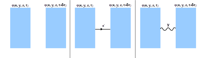
In other words in j-space, zero interaction means no change in the corresponding tangent field, or equally fine-structure constant α = 0 implies δφ = 0. Let us now assume that a simple interaction between an electron and a photon takes place, resulting in change in momentum of the electron. This interaction will result in a change in the field as shown below:
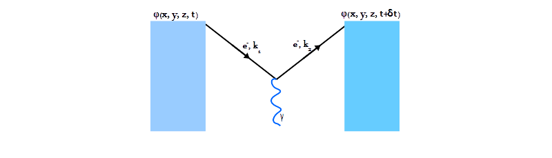
Here is an immediate problem. The measurements are made by Aku who being a macroscopic observer, will not be able to measure the change in field φ due to this simple interaction, as the change itself is very nearly in Planck's domain and well beyond Aku's measurement capacity. In fact it is almost certain that there are many more than one interaction, in the smallest time interval which can be precisely measured by Aku.
So how do we visualize the measurements made by Aku? We are forced to move away from "counting" and use some other analytical techniques to understand the experimental results. In fact, we are moving into the territories of Special Relativity, Path Integrals and Green Functions. Before we start introducing structures in j-space, we need to understand what information does quantum electrodynamics provide us, regarding the physical world represented by the region-I of Kruskal-Szekeres Coordinates.
___________________
1. Conventionally Aku is allowed access to region-III also, but we have different purpose for region-III in j-space. In j-space the picture shown for Kruskal-Szekeres Coordinates is in a 2-dimensional plane, without the 3-d light cone.
2. If Aku had to provide the description of the interior region-II as well, we can further postulate that the operators used by either Obsc or Aku, are zero-trace matrices representing convex surfaces (e.g. Pauli or Gell-Mann matrices). Adjoints exist, and the condition that the sum of probabilities equals to 1 or U †U = 1, is satisfied. Please note that the region-II represents Planck domain and hence any measurement made by Aku for this region, are #PE < 1 measurements. (#PE1 : Probability Equal to 1 measurement)
***

Previous Blogs:
Sigma-z and I
Spin Matrices
Rationale behind Irrational Numbers
The Ubiquitous z-Axis
Majorana
ZFC Axioms
Set Theory
Nutshell-2014
Knots in j-Space
Supercolliders
Force
Riemann Hypothesis
Andromeda Nebula
Infinite Fulcrum
Cauchy and Gaussian Distributions
b-Field & Lower Mass Bound
Incompleteness II
The Supersymmetry
The Cat in Box
The Initial State and Symmetries
Incompleteness I
Discrete Measurement Space
The Frog in Well
Visual Complex Analysis
The Einstein Theory of Relativity
***

Attribution — You must give appropriate credit, provide a link to the license, and indicate if changes were made. You may do so in any reasonable manner, but not in any way that suggests the licensor endorses you or your use. No additional restrictions — You may not apply legal terms or technological measures that legally restrict others from doing anything the license permits. This is a human-readable summary of (and not a substitute for) the license.
