| The Knot Formation in j-space |
|---|
| The Knot Formation in j-space |
|---|
Home |
The Trefoil KnotThe
objective is to develop an algebraic expression for
knots, knots which are not further reducible in the
discrete
measurement space of an macroscopic observer ObsM, or j-space.
It should be fairly obvious that the permanent
knots can only be formed when crossings are
alternately over and under. In this context,
please also
see the remark made by Professor Tait. If two crossings are
either consecutively over or consecutively under, then
they are equivalent to an unknot and hence they can be
removed from the knot diagram. The requirement of the alternating crossings also has an important ramification. The knots if they exist in a measurement space, represent the structures corresponding to a particle which can exist only in an excited quantum state. We can also say that the results derived from Knot-theory, correspond to the statistical and quantum-statistical measurement domains.
This process is similar to saying that all the possible knots in j-space, must be embedded in the trefoil knot space. We make similar statement in group theory, where we assert that most fundamental structure which can be measured, is the convex structure, which is represented by zero-trace Pauli Spin matrices. However in j-space knots, a convex structure is not possible as we are considering over- and under- crossings both. We are likely to get a structure of the following form, instead of a zero-trace 2×2 matrix:  . .
In this case the values of the exponents of the variables in the trace, should add up to zero. If we look at the trace, we can identify Laurent Polynomials as possible description for knot structures in j-space. In the following sections, we describe how to write polynomials in a discrete measurement space we call j-space, for a trefoil knot and its variations in terms of knot-orientation and reflection.
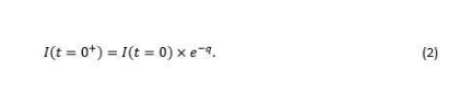
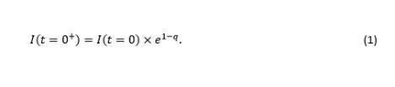 In Equation 1, q is a natural number (q = 1, 2, 3 ...), I(t=0) represents the information available for the initial state (t = 0), and I(t = 0+) represents the information available at a later instant, (t = 0+). A knot is formed when an observer cannot measure a state in a single measurement (single measurement represents zero entropy as loge1 = 0). In this case more than one measurement is needed and the entropy comes into the picture. We consider large q values where a statistical phenomenon is established. In that case Eqn. 1, is modified to,
We
postulate, that a knot is formed and a polynomial is
created, only when a measurement is made by a
macroscopic observer ObsM.
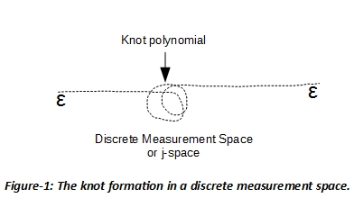
A finite capacity observer (v << c) is always
in a discrete measurement space. If a
state is below the observer's capacity threshold we
define it as ɛ, where ɛ represents an indeterminate
state for a finite capacity observer.
The knot formation in a discrete measurement space
is shown in Fig. 1.
Trefoil knot polynomials
A trefoil
knot as formed in a discrete measurement space for a
given q-value, is shown in Fig. 2. It is a
2-dimensional plane with third dimension representing
the motion within an infinitesimal ‘h’ along the
time-axis. We have the following properties
characterizing the knot,1. The motion along time-axis is in positive (over-crossing) and negative (under-crossing) directions both. This motion is along the perpendicular to the plane of the page. 2. The anticlockwise (ACW) or clockwise (CW) motions, are in the plane of the page. They represent the orientation of the knot at each crossing. 3. The order in which the crossing is approached is important. For example in Fig. 2, U2 and O3 cannot occur before O1. Similarly O3 cannot occur before U2. 4. The nature of the first crossing defines the knot as positive or negative. For example, if the first crossing of the knot is over-crossing (O1), the knot is classified as positive knot. Similarly, if the first crossing of the knot is under-crossing (U1), the knot is classified as negative knot.
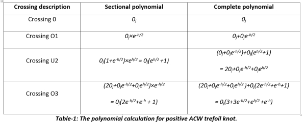
In calculating the polynomial the ACW orientation, is considered positive per trigonometric conventions. A sectional polynomial, represents the contribution of the specific crossing, which is then added to the contributions from the previous sections. The important part is the contribution of crossing 0. It is written as 0j to emphasize that in j-space to measure absolute zero, infinite capacity is required. Hence at best some minimum can be measured, which is represented as 0j. During calculation of polynomial the inclusion of 0j plays an important role. The polynomial is completed when a knot is formed. We define the polynomial variable as t = e-h. (Similar concept of knot thickening exists in conventional knot theory, except t in our case represents the absolute minimum distance an information string can shift along time-axis perpendicular to the 2D plane of the knot, in either direction. It is important to note that in j-space we are discussing a topological space, instead of the geometrical or physical space.) The polynomial for a positive ACW trefoil knot can be written from the Table-1 as,
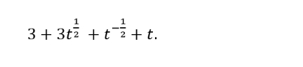
The normalized polynomial for a positive ACW trefoil knot is, 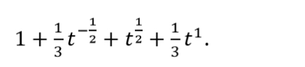 The coefficients of the polynomial take integer or fractional values. The polynomial variable t represents the variation of the information within the quantum ‘h’. 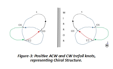 We can next consider the reflection of positive ACW trefoil knot, which will be positive CW trefoil knot (Fig. 3). In this case the orientation direction of the knot changes from ACW to CW, while the nature of over- and under-crossing and their respective order do not change. The plane of reflection can be either vertical or horizontal. In either case only change is in the orientation of the knot. The calculation of polynomial in this case is shown in Table-2. The CW orientation is negative per trigonometric convention. 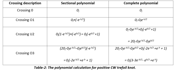 The polynomial for positive CW trefoil knot can be written as 3 - 3t1/2-t-1/2+ t where t = e-h. We can similarly write the corresponding polynomials for negative ACW and CW knots. The normalized polynomials for all four cases i.e. positive ACW, positive CW, negative ACW, and negative CW trefoil knots are summarized in the Table-3. 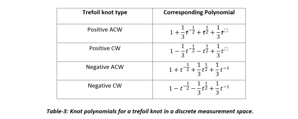 Additional PolynomialsWe can write a generalized algebraic expression for the normalized polynomials corresponding to the trefoil knot as in equation-3.  In eqn. 3, the coefficients (K1, K2, K3, K4) take the values (1/3, 1, 0, 1/3) for positive trefoil knot, and values (1, 1/3, 1/3, 0) for negative trefoil knot. The coefficients s1 and s2 take the values (1, 1) and (-1, -1) for ACW and CW orientations of the trefoil knot. We can write an additional set of the normalized polynomials for positive and negative trefoil knots for the values equal to (1, -1) and (-1, 1) for the coefficients (s1, s2) as shown in eqn. 4. The values of the coefficients (K1, K2, K3, K4) are left unchanged.
We
therefore have a set of eight normalized polynomials
for a trefoil knot in a discrete measurement
space. The physical interpretation of the
polynomials represented by eqn. 4, is yet to be
ascertained.
|
" It had for some time struck to me as very singular that, though I could easily prove that (when nugatory intersections are removed) a knot in which the crossings are alternately over and under is not further reducible ......" - Professor Tait in Proceedings of the Royal Society of Edinburgh, 1876-77. |